Case Study: Bayesian Networks

29 December 2003

This is a start towards a first cut at representing and searching for a Bayesian network or a causal network in the project inductive inference using Haskell (Allison 2003).

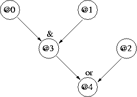
Figure 1 shows a very(!) simple network where attributes 0, 1 and 2 are independent "parents", and attributes 3 and 4 are dependent "children": @3 = @0 & @1, @4 = @2 or @3. In general, networks can be directed acyclic graphs (DAGs). Attributes can be discrete or continuous. Training data are usually "noisy".

Figure 1: Simple Network

A node with parents contains a function-model (regression); it models the child conditional upon its parents. Conditional probability tables (CPTs), i.e. finite function models, are often used in the case of discrete parents and children. If attributes have a high arity, or if there or many parents, or both, a full CPT can be very large with many parameters to estimate. Friedman & Goldszmidt (1996) suggested using decision-trees, i.e. classification trees, in place of CPTs within the nodes of networks. A classification tree can "become" a full CPT in the limit but can be much more economical, that is less complex, in many cases. A classification tree can also test continuous attributes and can have discrete or continuous distributions, or regressions, in leaves (e.g. Allison 2003).  Comley and Dowe (2003) have also used trees within the nodes of networks.

The [200309/] code already contains an estimator for classification trees which can handle discrete and/or continuous attributes. With just a little help, it can be used to estimate a Bayesian network as follows:

estNetwork  perm  estMV  dataSet =
 let n = length perm

     search _  []     = []  -- done

     search ps (c:cs) =     -- use parents, ps, to predict children, c:cs
      let opFlag  = ints2flags [c] n  -- identify the child, c, ...
          ipFlags = ints2flags ps  n  -- ... and the parents, ps.
          cTree = estCTree (estAndSelect estMV opFlag)  -- leaf estimator
                           (splitSelect ipFlags)        -- allowed tests
                           dataSet dataSet              -- !
      in cTree : (search (c:ps) cs)  -- i.e. a list of classification trees

     trees     = search [] perm                                  -- network
     msgLen    = sum (map msg1 trees)                            -- cost
     nlP datum = sum (map (\t -> condNlPr t datum datum) trees)  -- neg log Pr

 in MnlPr msgLen nlP (\() -> "Net:" ++ (show trees))        -- a Model

For simplicity only, estNetwork is given a permutation, perm, a total ordering of the attributes. (It would be easy to add a search for a best permutation. A search through all permutations would be slow, but some obvious heuristics suggest themselves, e.g. find for the best attribute, that gives the biggest information saving, to go last and repeat on a reduced set). estNetwork is also given an estimator, estMV, for a particular type of Model, and a training data set.

estMV is an estimator for a new kind of multivariate Model, ModelMV:

data ModelMV dataSpace =
  MnlPrMV ([Bool] -> MessageLength)              -- msg1
          ([Bool] -> dataSpace -> MessageLength) -- msg2
          ([Bool] -> String)                     -- Show
          Int                                    -- width

It is equivalent to an ordinary ModelType except that its abilities are qualified by a list of Boolean "flags" which can be used to turn attribute positions "on" and "off". The data type can be made an instance of classes Show, SuperModel and Model in the obvious way.

The flags are related to a new class Project. Anything that is project-able, i.e. an instance of Project, can behave like itself, whatever that is, on a select-ed subspace:

class Project t where
  select  :: [Bool] -> t -> t  -- non-selected parts become "identities"
  selAll  :: t -> [Bool]       -- i.e. all "on" flags

instance Project (ModelMV ds) where
  select bs (MnlPrMV m n s w) =
    MnlPrMV (\bs' -> m (zipWith (&&) bs bs'))
            (\bs' -> \datum -> n (zipWith (&&) bs bs') datum)
            (\bs' -> s (zipWith (&&) bs bs'))
            w

  selAll (MnlPrMV _ _ _ w) = replicate w True

It is necessary to create an estimator, estMV, that is specific to the type of data that the network models. It contains a suitable estimator for each attribute type, e.g. a multiState for a discrete attribute, and a normal (Gaussian), say, for a continuous attribute.

Looking back at estNetwork, notice how the search uses the elements of the permutation to select attributes as inputs (ip) or output (op) to the classification tree estimator estCTree. Also recall that estCTree requires a function that gives it options for splitting (partitioning) the input data space; this is the purpose of class Splits in [200309/]. For a Bayesian network, we need to be able to split on selected (by a list of Boolean flags) attributes, rather than on all attributes. As a stop-gap measure, a class Splits2 has been defined to enable this. If this turns out to be the "right" way to do things the abilities of Splits2 will probably be moved into Splits.

MML costing

It is assumed that the permutation is common knowledge. This would not be so if searching over all permutations and the cost of stating the permutation should then be added. The message length of a classification tree already includes the statement of the tests (splits, partitions) of the input attributes that it uses.

Discussion

Note that both discrete and continuous attributes can appear in the same network.

estCTree could be abstracted out so that the estNetwork algorithm could also work with conventional conditional probability tables (CPTs), or with other function-models, including continuous ones.

As it is, ModelMV, is more general than necessary (for estNetwork). Such a model can calculate the marginal distribution of any subspace of its data space which is easy in this case because the attributes are independent. It would be sufficient to be able to select, by an Int parameter, a single attribute to model. However, the present generality makes for a certain symmetry with the selection of input attributes and potentially allows, say, for two or more correlated "children" to be modelled in single node, which might be more economical in some cases although the search would be harder.

Some sort of template(?) Haskell might be able to generate automatically the estimator instance of ModelMV to match the type of the data.

In this example, perm = [0, 1, 3, 2, 4], e.g. @2 can potentially depend on none, some, or all of @0, @1 and @3; it turns out to be none:

Net:[
{CTleaf mState[0.48,0.52],_,_,_,_},                -- @0

{CTleaf _,mState[0.5,0.5],_,_,_},                  -- @1

{CTfork @1=False|True[
   {CTleaf _,_,_,mState[0.99,0.01],_},
   {CTfork @0=False|True[
      {CTleaf _,_,_,mState[0.98,0.02],_},
      {CTleaf _,_,_,mState[0.02,0.98],_}]}]},      -- @3 | @0,@1

{CTleaf _,_,mState[0.5,0.5],_,_},                  -- @2

{CTfork @2=False|True[
  {CTfork @3=False|True[
    {CTleaf _,_,_,_,mState[0.99,0.01]},
    {CTleaf _,_,_,_,mState[0.04,0.96]}]},
  {CTleaf _,_,_,_,mState[0.01,0.99]}]}]            -- @4 | @2,@3

The present result of estNetwork is a simple (multivariate) ModelType. It does implicitly contain the information necessary for "belief updating" and "intervention", but how best to package and implement them is undecided.

One wonders if `width' should be a property of many types -- ModelMV, tuples, etc. -- in which case maybe a class Width having an operator width might be appropriate.

The keen Haskell programmer will spot some instances of lazy programming, not lazy evaluation, that could be tidied up.

E.g., mixed

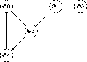
And just to show that it is possible, without requiring any new features, an inferred ``mixed'' example where @0 and @4 are continuous and @1, @2 and @3 are discrete (Boolean):

Net:[
{CTleaf N(1.0,0.41)(+-0.1),_,_,_,_},           -- @0 ~ N(1,0.4)

{CTleaf _,mState[0.5,0.5],_,_,_},              -- @1

{CTfork @0<|>=1.4[                             -- @2 | @0,@1
  {CTleaf _,_,mState[0.99,0.01],_,_},
  {CTfork @1=False|True[
    {CTleaf _,_,mState[0.98,0.02],_,_},
    {CTleaf _,_,mState[0.02,0.98],_,_}]}]},    -- i.e. (@0>1.4)&& @1

{CTleaf _,_,_,mState[0.5,0.5],_},              -- @3, a "dummy"

{CTfork @2=False|True[                         -- @4 | @0, @2
  {CTfork @0<|>=1.0[                           -- @2==False, test @0
    {CTleaf _,_,_,_,N(0.55,0.2)(+-0.1)},         -- @0 < 1.0
    {CTfork @0<|>=1.4[                           -- @0 >= 1.0, test
      {CTleaf _,_,_,_,N(1.0,0.2)(+-0.1)},          -- @0 [1.0,1.4)
      {CTleaf _,_,_,_,N(1.45,0.2)(+-0.1)}]}]},     -- @0 >= 1.4
  {CTleaf _,_,_,_,N(3.45,0.2)(+-0.1)}]}        -- @2 == True
]

104.1 nits

NB. Above, μs limited to [-10,+10], σs limited to [0.2,10.0]. Recall that N(_,_)(+-0.1) refers to data measurement accuracy.

Figure 2: Mixed Continuous (@0,@4) and Discrete (@1,@2,@3) Network

Lost Person

Note the modelling of "missing data" by "(Maybe 50:50<Model>?". (Note, fixed 50:50 was used because it was thought inappropriate to estimate missing-ness for this application.)

Net:[

@1 Age:
{CTleaf _,(Maybe 50:50,N(40.6,27.5)(+-0.5))...},

@2 Race =  White | Black:
{CTleaf _,_,(Maybe 50:50,mState[0.66,0.34])...},

@3 Gender = Male | Female:
{CTleaf _,_,_,(Maybe 50:50,mState[0.72,0.28])...},

@0 Tipe = Alzheimers| Child| Despondent| Hiker| Other| Retarded| Psychotic:
{CTfork @1(<|>=19.0|?)[
  {CTfork @3(=Male|Female|?)[
    {CTleaf (Maybe 50:50,mState[0.04,0.04,0.04,0.04,0.04,0.74,0.04])...},
    {CTleaf (Maybe 50:50,mState[0.11,0.11,0.11,0.11,0.11,0.33,0.11])...},
    {CTleaf (Maybe 50:50,mState[0.01,0.94,0.01,0.01,0.03,0.01,0.01])...},
  {CTfork @2(=White|Black|?)[
    {CTleaf (Maybe 50:50,mState[0.94,0.01,0.01,0.01,0.01,0.01,0.01])...},
    {CTleaf (Maybe 50:50,mState[0.89,0.02,0.02,0.02,0.02,0.02,0.02])...},
    {CTfork @3(=Male|Female|?)[
      {CTleaf (Maybe 50:50,mState[0.02,0.02,0.02,0.02,0.02,0.48,0.44])...},
      {CTleaf (Maybe 50:50,mState[0.03,0.03,0.03,0.03,0.03,0.40,0.45])...},
      {CTfork @1(<|>=63.0|?)[
        {CTleaf (Maybe 50:50,mState[0.02,0.01,0.65,0.23,0.01,0.01,0.04])...},
        {CTleaf (Maybe 50:50,mState[0.57,0.02,0.18,0.02,0.18,0.05,0.02])...},
        {CTleaf (Maybe 50:50,mState[0.14,0.14,0.14,0.14,0.14,0.14,0.14])...}]}]}]},
  {CTleaf (Maybe 50:50,mState[0.10,0.18,0.22,0.25,0.18,0.02,0.06])...}]},

@4 Topography = Mountains | Piedmont | Tidewater:
{CTleaf _,_,_,_,(Maybe 50:50,mState[0.17,0.52,0.31])...},

@5 Urban = Rural | Suburban | Urban:
{CTfork @4(=Mountains..Tidewater|?)[
  {CTleaf _,_,_,_,_,(Maybe 50:50,mState[0.93,0.04,0.04])...},
  {CTleaf _,_,_,_,_,(Maybe 50:50,mState[0.70,0.19,0.11])...},
  {CTleaf _,_,_,_,_,(Maybe 50:50,mState[0.38,0.02,0.6 ])...},
  {CTleaf _,_,_,_,_,(Maybe 50:50,mState[0.73,0.2 ,0.07])...}]},

@6 HrsNt:
{CTfork @1(<|>=62.0|?)[
  {CTleaf _,_,_,_,_,_,(Maybe 50:50,N( 8.7, 7.6)(+-0.5))...},
  {CTleaf _,_,_,_,_,_,(Maybe 50:50,N(21.4,26.3)(+-0.5))...},
  {CTleaf _,_,_,_,_,_,(Maybe 50:50,N(20.0,...1-case...)...}]},

@7 DistIPP:
{CTfork @6(<|>=1.0|?)[
  {CTleaf _,_,_,_,_,_,_,(Maybe 50:50,N( ...no-cases... )...},
  {CTleaf _,_,_,_,_,_,_,(Maybe 50:50,N(0.59,0.6)(+-0.2))...},
  {CTleaf _,_,_,_,_,_,_,(Maybe 50:50,N(1.52,2.8)(+-0.2))...}]}]

network: 115.1 nits, data: 5396.6 nits
null:   5935.6 nits (@0..@7)

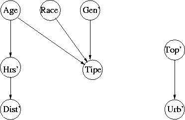
Figure 3: Lost Person Network, 8 Attributes

	@0: Tipe = Alzheimers | Child |... @1: Age   @2: Race   @3: Gender   @4: Topography   @5: Urban   @6: HrsNt   @7: DistIPP   @8: TrackOffset   @9: Health = Well | Hurt | Dead --after!   @10: Outcome = Find | Suspended | Invalid @11: FindRes = Ground | Air |...| Dog @12: FindLoc = Brush | Woods |... @13: HrsFind   @14: HrsTot
Approx. 9,700 nits (network+data) v. 10,400 nits (null+data).

Figure 4: Lost Person Network, all 15 Attributes

References

[All03] L. Allison. Types and Classes of Machine Learning and Data Mining. ACSC2003, pp.207-215, Adelaide, 4-7 February 2003.

[All04] L. Allison. Inductive Inference 1.1. TR 2004/153, School of Computer Science and Software Engineering, Monash University, May 2004.
Includes mixtures of time-series, and mixed Bayesian networks.

[CD03] J. W. Comley & D. L. Dowe. General Bayesian networks and asymmetric languages. Hawaii Int. Conf. Statistics and Related Fields (HICS #2), June 2003.

[FG96] N. Friedman & M. Goldszmidt. Learning Bayesian networks with local structure. UAI'96, pp.252-262, 1996.

 

Also see

[All06] L. Allison. A Programming Paradigm for Machine Learning, with a Case Study of Bayesian Networks, ACSC2006, pp.103-111, 2006,

and other [references] including TR 2004/153 'Inductive inference 1.1', TR 2005/177 and 'Inductive inference 1.1.2'.