| ^Bioinformatics^ ^#Alignment^ | > JME, 35, pp.77-89, 1992 [preprint.ps] > |
A preliminary version of this paper was presented at a joint session of the AAAI Spring Symposia on ``Artificial Intelligence and Molecular Biology'' and on the ``Theory and Application of Minimal Length Encoding'', at Stanford, March 27-29 1990.
A longer paper on the project titled ``Finite-State Models in the Alignment of Macromolecules'' later appeared in the Journal of Molecular Evolution, 35, pp.77-89, doi:10.1007/BF00160262, 1992.
* 1998:
now School of Computer Science and Software Engineering,
Monash University,
Australia 3168
Abstract: Minimum message length techniques are applied to problems over strings such as biological macromolecules. This allows the posterior odds-ratio of two theories or hypotheses about strings to be calculated. Given two strings we compare the r-theory, that they are related, with the null-theory, that they are not related. This is done for one, three and five-state models of relation. Models themselves can be compared and this is done on real DNA strings and artificial data. A fast, approximate MML string comparison algorithm is also described.
Keywords: alignment, edit distance, homology, inductive inference, MML, similarity, string.
Minimum message length (MML) encoding techniques are applied to inductive inference problems over strings derived from sequencing biological macro-molecules[Alli1]. The paper is framed in terms of DNA strings but the techniques apply to proteins and to other strings.
Given two strings, we consider the questions are they related and, if so, how are they related? We give algorithms to answer these questions for one, three and five-state models of relation. We also consider the question of which is the right model for a family of strings and give some results for DNA. A fast approximate MML algorithm is also described.
To illustrate the MML method of string comparison, consider a transmitter who must send two strings to a receiver. They may previously have agreed on any algorithms, codes and conventions to be used. The null-theory or hypothesis is that the strings are unrelated. In this case, the transmitter sends one string and then the other which requires approximately two bits per character. Conversely, the r-theory is that the strings are related. If the transmitter can find a "good" theory or hypothesis relating the characters of the two strings then it may be possible to encode them more succinctly. The transmitter then sends a message which states (a) the inferred theory and (b) encodes the strings using a code based on the theory. The MML method selects the theory giving the shortest message. A very detailed theory may allow a very short encoding of the strings proper but the details of the theory add to the message length. MML encoding thus defines an optimal degree of detail in this trade off.
It is assumed that any one string is random in the sense of Kolmogorov complexity[Chai][Kolm][Li]. This is nearly the case for biological macro-molecules and it is difficult to encode a typical DNA string in much less than two bits per character. This assumption is not essential to the MML method in principle but makes its application easier. There is for example an echo of a presumed purine-any-pyrimidine (RNY) ancient genetic code[Shep] which could be accommodated by considering codons to be the characters within strings.
We relate strings by simple generation and mutation machines and consider one, three and five-state machines in detail.
If accurate prior probabilities for strings and relations are known, an optimal code can be designed for them. The minimum message length is minus log2 of the probability of the event described. Often such probabilities are not known in advance but a model having one or more parameters can be agreed on. A message must include the parameter values and the best values give the shortest message. Two hypotheses can be compared on the basis of message lengths and the difference in message lengths is minus log2 of their posterior odds-ratio. Because a natural null-theory exists, this leads to hypothesis testing. No hypothesis having a message length longer than the null-theory is acceptable.
There are practical and theoretical advantages to MML encoding as a method of inductive inference. It keeps us honest in that anything not agreed to apriori must be included in the message. When real-valued parameters are involved, it implies an optimal degree of precision for their estimates. It is invariant under monotonic transformation of parameters. It focuses attention on the language being encoded, on what it can express and on the probabilities of messages. When accurate prior probabilities are not known, all the techniques and heuristics of data-compression and of coding theory[Hamm] can be used to get a good code. MML encoding is safe in that the use of a suboptimal code cannot make a theory appear more acceptable than it should be.
Note that in practice no encoding actually takes place; we simply calculate what the message length would be if encoded. Note also that arithmetic coding[Lang][Witt] is capable of transmitting information in fractions of a bit.
MML string comparison is closely related to maximum-likelihood methods. An important difference is that MML methods fully cost the model complexity. Felsenstein[Fels] gave a maximum-likelihood method to infer an evolutionary tree for a family of strings in the absence of insertions and deletions, or when the insertions and deletions are given externally. Bishop et al[Bish2] gave a maximum-likelihood method to infer the time since two related strings diverged. It is similar to our MML method for a one-state model. Bishop and Friday[Bish1] note that "there is as yet no formally developed method for assessing the significance of the difference in the likelihoods (of two different [phylogenetic] trees)." The MML method does not suffer from this problem and has a formal interpretation of differences in message length and indeed has a rigorous test of statistical significance. Reichert et al[Reic][Cohe][Wong] considered the brief encoding of pairs of strings under a single model of relation but did not compare models.
Solomonoff[Solo] proposed MML encoding as a basis for inductive inference.
Wallace and Boulton[Wall1] first applied it
in producing a practical classification algorithm.
Georgeff and Wallace[Geor] give a good introduction to MML methods
and Wallace and Freeman[Wall2] describe the
statistical foundations.
|
|
|
There are many ways of explaining or modeling two strings given that they are related. In the mutation model, a simple machine reads one given string and a sequence of mutation instructions while writing the second given string (figure 1).
string A:     TATACGTTACAC
instructions: copy, copy, ins(A), copy, copy,
              change(G), change(C),
              copy, copy,
              del, copy, copy, copy, ins(A)
string B:     TAATAGCTTCACA
Figure 1: Mutation Model Example.
|
In the generative model, a different simple machine reads a sequence of generative instructions while writing the two given strings in parallel (figure 2).
instructions:
  match(T), match(A), ins(A),
  match(T), match(A),
  change(C,G), change(G,C),
  match((T), match(T),
  del(A), match(C), match(A),
  match(C), ins(A)

string A: TATACGTTACAC
string B: TAATAGCTTCACA
Figure 2: Generative Model Example. |
Note that for traditional reasons we use the terms `change' when a different character appears in each string, `delete' (del) when a character appears in string A and not in string B and `insert' (ins) when a character appears in B and not in A under both models but with appropriate meanings. For both models, a given sequence of instructions is equivalent to a traditional alignment, see figure 3.
string A: TA-TACGTTACAC-
          || ||  || |||
string B: TAATAGCTT-CACA
Figure 3: An Alignment.
|
It is therefore clear that the mutation and generative models are equivalent and we usually prefer the generative model on grounds of symmetry. We use the terms `alignment' and `instruction sequence' interchangeably.
Note that alignments and sequences of generative or mutation instructions are not unique. Often we want an optimal explanation, alignment or instruction sequence but even suboptimal explanations may be plausible.
Given two macro-molecules, A and B, it is often assumed
that they evolved independently from a common ancestor P.
We could model this by two mutation machines, MA and MB,
which each read P and their own instruction sequence and produced
A and B respectively.
A and B have infinitely many possible ancestors P
but most are wildly improbable.
Summing over all possible P gives the probability
of A and B being related under this model.
If we knew P and the instruction sequences for MA and for MB,
the sequences could be synchronised to derive an alignment or
an instruction sequence for a single generation machine.
An alignment corresponds to a set of possible
ancestors (figure 4).
Alignment 1: TA-TACGTTACAC-
             || ||  || |||
             TAATAGCTT-CACA

Ancestors 1: TA[A-]TA[CG][CG]TT[A-]CAC[A-]


Alignment 2: T-ATACG-TT-ACAC
             | ||| | || |||
             TAATA-GCTTCACA-

Ancestors 2: T[A-]ATA[C-]G[C-]TT[C-]ACA[C-]
Figure 4: Alignments and Possible Ancestors.
|
Therefore the r-theory should not be based on just one alignment but summed over all of them. We can decide if A and B are related but P must remain uncertain unless extra information is provided. Note that there may have been characters in P that were deleted in both A and B and for which no direct evidence remains. Note also that the assumption of a constant rate of evolutionary mutation implies that MA and MB are equal and it is difficult to see how one could make any other assumption given just two strings.
Traditional alignment programs[Bish3][Sank][Wate] select alignments that have a minimum cost, or equivalently a maximum score, under some measure. The minimum message length principle implies that the cost of an alignment should be the length of a message under an optimal code for alignments. To answer the question, are A and B related, all alignments should contribute according to their probability. The corresponding message and its code should transmit A and B given that they are related; it should not transmit a single alignment.
Our models and codes may have parameters for the form of a generative machine and the probabilities of its instructions which must be included in the message. In this way simple and complex models may be compared on an equal footing. In following sections we specify and compare one, three and five-state models.
The one-state generative machine has a single state and transitions or instructions of the following forms: match(ch), change(ch1,ch2), ins(ch), del(ch). The match instruction generates the same character `ch' in both strings. The change instruction generates ch1 in string A and ch2 in string B. The insert (ins) instruction generates a character in string A and the delete (del) instruction generates a character in string B. A single instruction having probability `p' is optimally encoded in -log2(p) bits plus two bits for each character, except that the two characters in a change are different and together require log2(12)<4 bits. Often we require that P(ins)=P(del). The probability of a sequence of instructions of fixed length is the product of the probabilities of individual instructions and the message length of the sequence is the sum of the message lengths of the instructions.
If the probabilities of instructions are known apriori,
a fixed code can be based on them.
The dynamic programming algorithm (DPA)
is modified to compute the message length
of an optimal instruction sequence (figure 5).
Boundary Conditions:
   D[0, 0] := 0
   D[i, 0] := delete * i,  i:=1..|A|
   D[0, j] := insert * j,  j:=1..|B|

General Step, i:=1..|A| and j:=1..|B|:
   D[i,j]:=min(D[i-1,j  ] + delete,
               D[i  ,j-1] + insert,
               D[i-1,j-1] +
                 if A[i]=B[j] then match
                              else change)
Figure 5: Dynamic Programming Algorithm.
|
Each instruction is given a weight based on -log2 of its probability. Note that a match does not have zero cost. D[i,j] is the message length of an optimal sequence to generate A[1..i] and B[1..j]. It has been shown[Alli2] how to normalise Seller's[Sell1][Sell2] and similar metrics so as to extract the probabilities implicit in them [See also L.Allison, Jrnl. Theor. Bio. 161, pp263-269, 1993]. Ignoring the matter of coding lengths and parameter values for now, the algorithm finds an alignment or instruction sequence having the minimum message length.
When probabilities are not known in advance, they must be inferred from the strings. A simple iterative approach finds at least a local optimum. Initial probabilities are guessed and an alignment is found. New probabilities are calculated from the frequencies of instructions in the alignment and used in the next iteration. The process quickly converges. The inferred parameter values are included in the message; Boulton and Wallace[Boul] give the necessary calculations.
The length of a sequence is not known in advance and must be included in any message. In the absence of more information we use Rissanen's[Riss] universal log* prior to transmit the length.
The overhead of transmitting the length of an instruction sequence and the parameter values becomes a smaller fraction of the total message length as string length increases. Since the DPA does not consider the overhead when finding an alignment, the overall result is not guaranteed to be optimal. In practice it is, particularly for reasonably long strings.
Optimal alignments are not unique in general. Even suboptimal alignments make some contribution to the r-theory. The `min' in the DPA (figure 5) chooses the single alignment having the smallest message length, the largest probability. If the probabilities are instead added, for they correspond to exclusive events, then D[i,j] is the (-log2) probability that A[1..i] and B[1..j] arose through being generatively related by the machine but in some unspecified way. This yields the probability of A and B given the r-theory. The addition of probabilities is a probabilistic argument but a corresponding code has been devised by Wallace[Wall3]. It reduces the message length of the r-theory below that of a single alignment. When instruction probabilities are not known they must be inferred. The same iterative search is used, weighted frequencies being added when alternative sequences are combined and their probabilities added.
The null-theory is that A and B arose independently and this is the complement of the r-theory. The null-theory is encoded by encoding string A and then encoding string B. It must include their lengths. Rather than transmit two lengths, we transmit the sum of the string lengths using the universal prior and the difference of the lengths using a binomial prior. This is reasonable because random insertions and deletions perform a random walk on the difference of the lengths. If P(ins)=P(del)=1/2, the null-theory and the r-theory have the same prior over |A|-|B|. If P(ins)=P(del)<1/2, the r-theory has a tighter distribution on |A|-|B|.
The odds-ratio of the r-theory and the null-theory is the binary exponential of the difference in their message lengths. Since they are complementary, their posterior probabilities can be calculated.
Running the r-theory in reverse,
D'[i+1,j+1] is (-log2) the probability of
A[i+1..|A|] and B[j+1..|B|] being generated.
Thus, D[i,j]+D'[i+1,j+1] is the (-log2) probability
of A[1..i] and B[1..j] being generated
and A[i+1..|A|] and B[j+1..|B|] being generated
and is proportional to the probability of the "true"
alignment partitioning the strings in this way.
A density plot of this function
is a good way of visualising possible alignments
(figure 6).
|
See:
Allison, Wallace & Yee,
[AIM'90], and
for grey-scale alignment probability plots.
    T A A T A G C T T C A C A
   $ - - .
T: - $ # - . .
A: . - $ $ - . . .
T: . . - - $ - - . .
A:   . . - - $ # - . .
C:     . - - # + # - . .
G:     . . . - # $ + . .
T:       . . . - + $ + - .
T:         . . . . + $ # - .
A:           . . . - # - # - .
C:               . . - # - # -
A:                 . . - # + #
C:                     . - # $

key     :   $  #  +  -  .
MML plus: 0..1..2..4..8..16 bits

null-theory=62.4  r-theory=58.5
probability related=0.94
Figure 6: Alignment Densities.
|
Note the areas of uncertainty where there are multiple reasonable
explanations, CG:GC and ACAC:CACA.
In this example the r-theory is certainly acceptable
but any single alignment is at best marginally acceptable.
The density plot is a "fuzzy" alignment.
It is a good representation of the possible ancestors of A and B
for use in multiple string alignment
or in phylogenetic tree reconstruction[Alli3].
We note that string alignment algorithms
employing linear costs w(L)=a+b*L for indels of length L
are in common use.
The constant `a' is a start-up cost to discourage the inference of
many short block indels
and is thought to be realistic for macro-molecules.
This can be modelled by a three-state machine (figure 7).
states:
   S1: match/change state
   S2: insert state
   S3: delete state

transitions:
   S1--match--->S1  S1--change-->S1
   S1--insert-->S2  S1--delete-->S3
   S2--match--->S1  S2--change-->S1
   S2--insert-->S2  S2--delete-->S3
   S3--match--->S1  S3--change-->S1
   S3--insert-->S2  S3--delete-->S3

conservation:
   p(m|Sj)+p(c|Sj)+p(i|Sj)+p(d|Sj)=1,
   j=1,2,3
Figure 7: Three-State Machine. |
When P(ins|S1)<P(ins|S2) there is a low start-up probability, a high start-up cost, on block indels. A linear cost function corresponds to a geometric prior on indel lengths, for -log2(pLq) = -log2(q) - log2(p)*L.
Gotoh[Goto] has given an algorithm to infer an optimal alignment for linear weights. Briefly, the DPA is modified to maintain three values in each cell of the D matrix. One value corresponds to each state. As before, we have further modified the algorithm to add probabilities. Again probabilities must be inferred from the strings if they are not known apriori. The iterative scheme described previously is used.
The algorithm is run forward and backwards and results added to produce alignment density plots. The three-state model has more parameters than the one-state model and these add to the length of the header part of the r-theory message.
Gotoh[Goto] also provided an algorithm
to find a single optimal alignment under
piece-wise linear indel costs.
Bilinear indel costs can be modelled by a five-state machine
(figure 8).
states:
  S1: match/change state
  S2: (short-)insert state
  S3: (short-)delete state
  S4: long-insert state
  S5: long-delete state

transitions:
  S1, S2, S3 as before plus
  S1--long-ins-->S4  S1--long-del-->S5
  S4--long-ins-->S4  S4--end-long-->S1
  S5--long-del-->S5  S5--end-long-->S1

conservation:
  p(m|S1)+p(c|S1)+p(i|S1)+p(d|S1)+
  p(long-ins|S1)+P(long-del|S1)=1  etc.
Figure 8: Five-State Model. |
We have modified the DPA to maintain five values, one for each state,
in the D matrix.
This kind of model is appropriate if
short indels are thought to be relatively frequent and
long indels rather infrequent which might account for point mutations
and larger events, perhaps introns/exons.
A fully-connected five-state machine would have a very large number of
transitions and parameters.
To reduce this we simply augment the three-state machine with
long-insert and long-delete states connected only to
S1.
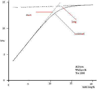 short: Ps(L)=0.098 x 0.50(L-1)x0.50
long: Pl(L)=0.002 x 0.98(L-1)x0.02 combined: Pc(L)=Ps(L)+Pl(L) Figure 9: Combining Length Costs of Long and Short Indels. |
As before, probabilities of alternative sequences are added. Note that because of this a medium length indel is considered to be partly long and partly short. Resulting indel costs are smooth and asymptotically linear; figure 9 gives an example.
The search for optimal five-state parameter values is more difficult. Because long-indels are expected to be rare they are initially given a low probability, a large start-up cost, but a high probability of continuation. A further useful strategy is to run the three-state model first and base initial probabilities for S1, S2 and S3 on the results with minor adjustments to conserve probability. The iterative process is used from this starting point.
Note that a special case of five-state data
is when the long indels occur at the ends of one or both strings,
when string A=A1;A2;A3 and B=B1;B2;B3
where A2 and B2 are related by a three-state-model and
A1, A3, B1 and B3 are unrelated, possibly null.
This amounts to looking for a common pattern A2:B2 in A and B.
This situation is rather common because interesting
pieces of DNA from a chromosome may have flanking regions
attached.
|
The one, three and five-state algorithms were run on both artificial data and real DNA strings.
The cost of stating the parameters of a model is a decreasing fraction
of the total message cost as string lengths increase.
For short strings, this may cause a simpler model to be favoured.
To study this effect, pairs of strings of various lengths
were generated by a five-state model
with various known parameter values.
For each setting, a collection of 15 to 30 pairs was generated.
For each model and collection, the r-theory algorithm was run
and the message lengths averaged.
This was done for the one, three and five-state
models.
S1 (match/change):
 P(match)=0.8  P(change)=0.000001
 P(short insert)=P(short delete)=0.098
 P(long  insert)=P(long  delete)=0.002
S2 (short insert):
 P(match)=0.49 P(change)=0.000001 (return to S1)
 P(short indel)=0.5  P(short delete)=0.01
S3 (short delete): similar to S2
S4 (long insert):
 P(long insert)=0.98
 P(end long)=0.02   (return to S1)
S5 (long delete): similar to S4

average short indel length = 2
average long indel length = 50
Table 1: 5-State Parameters for Generating Test Data. |
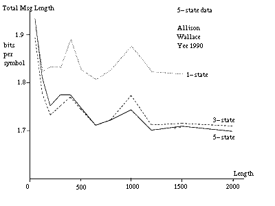
Figure 10(a) [see Allison et al 1992] gives plots of the total message lengths per symbol versus string length for strings generated by a five-state model having parameters indicated in table 1. In this case the probability of changes was held very low to isolate the interaction between short and long indels. There is a cross-over from favouring the three-state to favouring the five-state model at a string length of 500 to 1000 characters. (The inference for long strings is stronger than might be immediately apparent because the cost per symbol is plotted.) A single pair of strings from an unknown source and shorter than this cannot be identified as coming from a five-state rather than a three-state model.
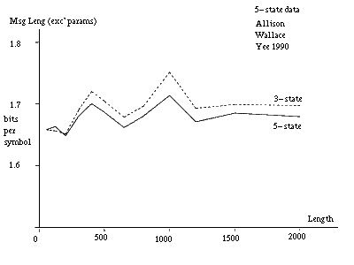
A pair of strings longer than 500 to 1000 characters can be identified as coming from a five-state model. Many pairs of shorter strings, assumed to be generated by the same model and parameter values, can also be so identified. It is sufficient for the parameter values of the pairs to be related rather than identical in this latter situation so that they need not be stated in full for each pair. To indicate what would happen in an extreme case of this situation, figure 10(b) gives message lengths under the three models when parameter costs are excluded. The data is the same as for figure 10(a). In this case, the cross-over from the three-state to the five-state inference is at about 150 characters for the given parameter values. At this point a pair is reasonably likely to have at least one long insert or delete for the given parameter values.
Note that the DNA coding regions for many proteins have lengths in the difficult range of 500 to 1000 characters. Note that the cross-overs would occur at shorter lengths for an alphabet size larger than 4.
When the similarity within each pair of strings is increased, the general picture is as described above but the cross-overs occur at greater string lengths. Increasing similarity favours simpler models. In the extreme case, two identical strings are best described by the one-state model.
It is clear that to draw any general conclusions about
the "true" model for real DNA, a pair of very long related strings or
a large number of pairs of related strings is required.
Such data are hard to come by
The Blur sequences are members of the large Alu family[Bain].
The typical Blur sequence is about 280 characters long.
               1-state  3-state  5-state
               ------------------------->model
Blur8  :Blur13    1039      946      943
                 (1016)    (912)    (909)
Blur11 :Blur13    1179      963      957
                 (1155)    (928)    (922)
Blur11':Blur13'    825      830      836
                  (801)    (800)    (802)
Lengths in parentheses are exclusive of parameter costs.
Table 2: Message Lengths in bits for some Blur Sequences. |
Table 2 gives some results of the one, three and five-state models on Blurs 8, 11 and 13. When whole strings are compared, the evidence strongly supports either the three or five-state model rather than the one-state model. The three and five-state models give message lengths within a few bits of each other which is insufficient to conclude in favour one rather than the other. Blur11' and Blur13' were derived by forming an alignment and truncating any terminal overhanging segment on either string. Results for this pair slightly favour the one-state model suggesting that the overhangs were the dominant factor in the whole strings. The difficulty is probably that the Blur's are too short. There are many Blurs but it is not known how they are related. We suggest that the correct way to explain them is by an MML multiple alignment with respect to a phylogenetic tree (or forest). Algorithms for this problem are the subject of current work [e.g. see Allison & Wallace, Jrnl. Molec. Evol. 39 pp418-430, 1994].
The globin genes and pseudogenes are often used in phylogenetic studies
of primates[Holm].
                 1state 3state 5state
                 --------------------
HSBGLOP:ATRB1GLOP 6414   6004   6007 inc' param's
                 (6383) (5960) (5958)exc' param's
Genbank id HSBGLOP: human beta type globin pseudogene 2153bp.Genbank id ATRB1GLOP: owl monkey psi beta 1 globin pseudogene 2124bp. Table 3: Message Lengths (bits) for 2 Globin Pseudogenes. |
Table 3 gives the results of the r-theory algorithms of the three models on human beta type globin pseudogene and owl monkey psi beta 1 globin pseudogene. The three and five-state models give similar results and the one-state model performs significantly worse.
The above results strongly suggest that the one-state model is not the correct one to use with DNA. They do not distinguish between the three and five-state models. It is clear that a great many more tests are required to discover if one of these, or some other model, is the correct one to use.
The basic DPA takes O(|A|*B|) time and space.
If a single optimal MML alignment is required,
Hirschberg's[Hirs] divide and conquer technique
can be used to reduce the space complexity to O(|B|).
This is not applicable if the MML of the r-theory is required.
Observations of alignment density plots (figure 6)
indicate that most of the probability is concentrated in a narrow region.
Fast approximate MML algorithms can take advantage of this
fact.
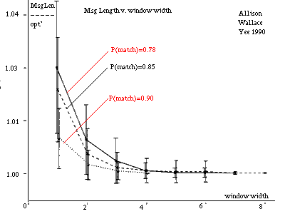 Figure 11: Message Length v. Window Size (approx'n algorithm). |
An approximate three-state algorithm has been programmed. Firstly, Ukkonen[Ukko] gave an O(|A|*D(A,B)) edit-distance algorithm for Seller's metric. This is fast for similar strings. The algorithm does not calculate the D matrix directly but rather the location of contours in it. The algorithm halts when a contour reaches D[|A|,|B|]. We applied Ukkonen's technique to linear indel costs. Secondly, as mentioned in section 3, arbitrary costs in a metric can be normalised to yield instruction probabilities. This process can be reversed to choose integer weights corresponding to "reasonable" probabilities. This is used to find an optimal alignment. Finally, a window containing all D cells that lie within a diagonal distance `w' of the optimal alignment is formed and the r-theory algorithm is run only within this window. All cells outside this window are considered to have probability zero and an infinite message length. The time and space taken for this step is O(max(|A|,|B|)*w). A graph of message lengths against w is given in figure 11 [see Allison et al 1992]. The random data was generated by a three-state model. The dominant influence on required window size is the probability of a match in state 1 which is indicated. It can be seen that a small window includes almost all the probability. This windowing technique could be applied to other models.
We have solved the question of two strings being related (the r-theory) for one, three and five-state models of string relation. The biological validity of such models is open to debate but we note that one and three-state models are implicit in alignment algorithms in common use. A major advantage of a formal model is that its assumptions are explicit and available for scrutiny and modification. We have given an objective method of comparing models of relation over a given set of strings and have applied it to the one, three and five-state models. The tests performed are only a first step and the models can be elaborated to account for unequal probabilities of changes, effects of codon bias, the genetic code and so on. The assembly of a large body of real biological test data remains a problem.
In general, a single alignment is excessively precise. All alignments are possible; some are more probable than others. The r-theory should include them all.
Modulo normalisation, an arbitrary cost function w(L) on blocks of matches, changes, inserts or deletes of length L implies a prior probability distribution 2-w(L) on run lengths. Problem specific knowledge can be used to design a good prior. Conversely if a cost function gives results judged (externally) to be good, it gives information about good priors and mechanisms relating strings.
A piecewise linear cost function on runs of instructions implies a finite-state machine or model. All such models have an O(|A|*B|) MML algorithm for the r-theory and for alignment probability densities. However, the number of transitions in the machine and thus the complexity of the algorithm rapidly increases with the number of linear segments making the cost function. Miller and Myers[Mill] have given an O(|A|*B|) or O(|A|*B|*log(max(|A|,|B|))) algorithm to find a single optimal alignment for arbitrary concave functions. There does not seem to be an r-theory algorithm or a density algorithm with this complexity for such functions.
Given a single pair of strings from an unknown source,
over an alphabet of size four
and of length less than 500 to 1000 characters
it is not possible to identify them as being the products of a five-state
process even if they are.
Longer strings or many pairs of shorter strings generated by
the same five-state process can be so identified.