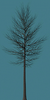
A stream with vegetation (Deussen et al SIGGRAPH 98)
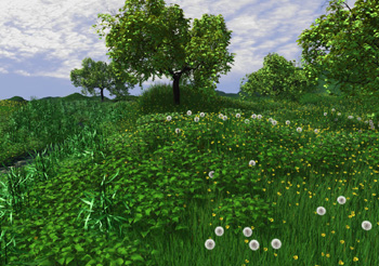
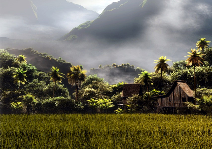
Bali 2005, Vue 5 Infinite demo. image
Lectures 3&4
|
|
A stream with vegetation (Deussen et al SIGGRAPH 98) |
Bali 2005, Vue 5 Infinite demo. image |
Prusinkiewicz, P, Lindenmeyer, A, Hanan, J.
"Developmental Models of Herbaceous Plants for Computer Imagery Purposes"
Computer Graphics, Vol 22 No. 4, August 1988 (SIGGRAPH 88), ACM Press, pp141-150
Prusinkiewicz, P, Lindenmeyer, A.
"The Algorithmic Beauty Of Plants",
Springer Verlag, 1990 [Available
in PDF format]
Prusinkiewicz P, Hammel M, Mjolsness E.
"Animation Of Plant Development"
Computer Graphics, SIGGRAPH 93, ACM Press, pp351-360
"Visual Models of Morphogenesis" (website)
Examples on the Algorithmic Botany website in animation format.
How is an L-grammar specified?
An L-System consists of:
|
V, a set of symbols called the alphabet of the grammar representing the modules of the plant; |
|
W, an axiom or initial string consisting of symbols from the alphabet representing the first module of the plant; |
|
P, a set of production rules to be applied in parallel to the axiom and symbols of the subsequent strings. Production rules replace a symbol, the predecessor module, with zero, one or several successor modules. |
Now, how about some examples?
|
K = {V, W, P} |
|
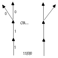
FIG. A sample visual representation of the string: 11[0]0
| K = {V,
W, P} V = {0, 1, [, ] } W = 0 P = p1: 0 ->11[0][0] p2: 1 -> 1 p3: [ -> [ p4: ] -> ] |
|
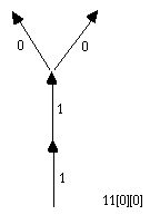
FIG. A sample visual representation of the string: 11[0][0]
A further example...
 |
 |
|
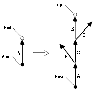
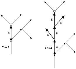
A visual representation of a tree production P. |
Application of P to edge S in tree 1. |
| a path: l | (the left context) |
| an edge: S | (the strict predecessor) |
| an axial tree: r | (the right context) |
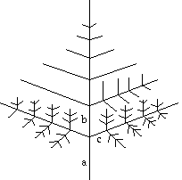
The asymmetry between l and r reflects the asymmetry in the neighbourhood of a module. Ie. There is only one path leading from the root of the tree to a given module, but each module may be the parent of a complete subtree.
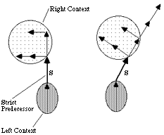
FIG. The satisfaction of a context-sensitive grammar.
Where exactly one production matches each possible instance of a symbol (or
in the case of context-sensitive grammars, set of symbols) we have
a deterministic L-System. (As in all the examples above.)
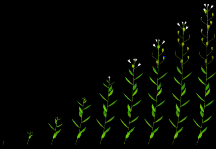
Development of Shepherd's Purse. (Prusinkiewicz et. al 1988)
Shepherd's Purse can be represented by a non-deterministic, parametric
L-system as follows.
| K = | {V, W, P} |
| V = | {A, B, F, I, L [, ] } |
| W = | A |
| P = | p1: A -> I0
[ L0 ] A p2: A -> I0 [ L0 ] B p3: B -> I0 [ L0 F0 ] B p4: Xi -> Xi+1 where i>=0 and X is an element of {I, L, F} |
Production p1 describes the initial vegetative growth of (L)eaves and (I)nternodes from apex A.
At some point in time as determined by one of the methods below, p1 is replaced by p2. This changes the Apex to its (F)lowering state.
From this point on, flowers are produced by p3 instead of leaves as previously.
The consecutive steps of I, L and F represent the parametized stages of development of an individual Internode, Leaf and Flower respectively.
An L-system can be used to represent the development of leaves, flowers and other plant organs by encoding the lengths, curves, number of petals, leaf veins etc. in alphabetic symbols of the grammar.
Eg. A vector may be repetitively scaled using a production rule: X -> SX
L-Systems may be used to model fractal plants, however, simpler fractal/graftal
models of plants are available.
Oppenheimer P.E.,
"Real Time Design and Animation of Fractal Plants and Trees"
Computer Graphics, Vol 20 No. 4, August 1986 (SIGGRAPH 86), ACM Press, pp55-64
|
a = 1.0 branch/stem ratio |
 |
|
Greene, Ned
"Voxel Space Automata: Modeling With Stochastic Growth Processes In Voxel
Space"
Computer Graphics Vol 23, July 1989 (SIGGRAPH 89), ACM Press, pp175 - 184
Greene (SIGGRAPH 1989)
Seed Locations
seed 0.5 -0.89 0.56
seed 0.35 -0.89 0.56
Skeleton Parameters
random tree {
| length |
2.4 |
limb length in voxel widths |
| branch_age_range |
1->3 |
1,2 or 3 iterations before branching (random) |
| branch_angle |
60 |
degrees |
| vertical_bias |
0.08 |
slight bias to grow upward |
| no_of_trials_max |
300 |
300 randomly perturbed trials before giving up |
| no_of_trials_min |
150 |
150 trials before selecting best proximity fit |
| seekprox |
1.5 |
pick trial with average proximity closest to 1.5 voxel widths |
| maxprox |
3.0 |
reject trials with average proximity greater than 3 voxel widths |
}
Illumination Parameters
light {
| blend sun | 0.8 |
blend sun exposure |
| blend sky | 0.2 |
blend sky exposure |
| exposure_min | 0.3 | nodes with <30% exposure become inactive |
| exposure_max | 1.0 | nodes with up to 100% exposure may be active |
| boost | 1.8 | 100% exposed nodes grow 1.8x faster than those with 30% exposure |
|
number_of_trials |
30 | attempt placement 30 times before giving up |
|
expected frequency |
1.5 | try to place 1.5 leaves per branch segment |
model
{
} |
co-ordinates
of polygonal leaf model ... |
The amount of light falling into a voxel consists of two components.
1. The sky exposure for a voxel:
2. The sun exposure for a voxel:
The different effects of Sun/sky exposure are weighted according to whether or not the plant responds well to diffuse or direct light.
 Greene (SIGGRAPH 1989) |
|
...a place for plants to grow
Watt, Watt
"Advanced Animation and Rendering Techniques, Theory and Practice"
Addison-Wesley 1992, Section 7.1, pp203-205
Foley, van Dam, Feiner, Hughes,
"Computer Graphics, Principles and Practice"
2nd edn, Addison-Wesley, 1987, Section 20.3, pp1020-1026
Kajiya, J.T,
"New Techniques for Ray Tracing Procedurally Defined Objects"
SIGGRAPH 83, pp91-102
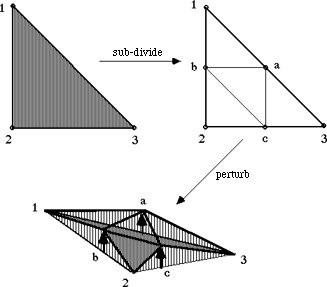 |
The ever-popular
fractal landcape may be simply constructed...
|
|
A height map may be used to add the effect of rock strata or snow-capped peaks. For example... |
 |
Snow on top, |
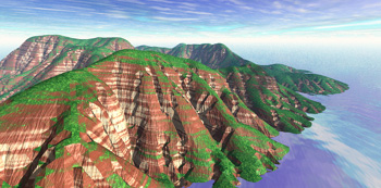 |
Foliage may also be simulated by appropriately colouring polygons with their normals within some range of the vertical (and their height below the snow-line). |
Useful for virtual rain to make virtual trees grow, and even for modelling
leaf clusters or grass. (Not forgetting to mention its use for modelling fireworks!)
Watt, Watt
"Advanced Animation and Rendering Techniques, Theory and Practice"
Addison-Wesley 1992, Section 18.1, pp415-417
Foley, van Dam, Feiner, Hughes,
"Computer Graphics, Principles and Practice"
2nd edn, Addison-Wesley, 1987, Section 20.5, pp1031-1034
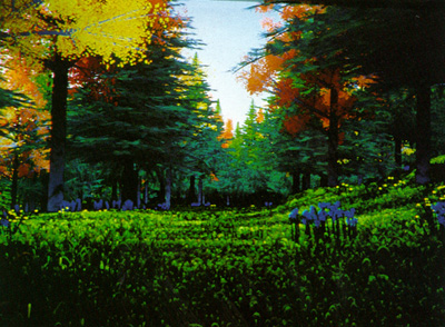 |
Image from The Adventures of Andre and Wally B. (Lucasfilm) 1984. Leaves and grass generated by particle systems. |
 |
 |
|
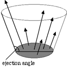
Particle emission from circular generation shape.
|
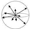
Particle emission from point (or spherical) generation
shape.
|
lecture notes | home
All material accessed from www.csse.monash.edu.au/~cema
is
© Copyright 1994-2008 Alan Dorin, Jon McCormack & Monash University
except where noted.