Lectures 9&10
Cells & Pix-cells (Pixels)
|
1. Cellular Automata
References & Reading Material:
Burks, A.W. (ed)
"Essays On Cellular Automata",
University of Illinois Press, 1970.
Gardner, M.
"The Fantastic Combinations of John Conway's New Solitaire Game, 'Life'",
Scientific American 223(4), pp120-123, 1970
Langton, C.G.,
"Studying Artificial Life with Cellular Automata",
Evolution, Games & Learning - Models for Adaptation in Machines & Nature,
(eds) Farmer et al, Fifth Conf. On Non-linear Systems, North-Holland,
pp120-149, 1985
|
What are Cellular Automata?
- Finite State Machines (FSM's) on an infinite grid.
- An FSM is connected only to its neighbour cells.
- An FSM's states are updated in parallel at discrete time intervals.
- The state of an FSM at time step t+1 is determined by the transition table
of the FSM.
- There must be a valid transition for each of the possible combinations of
the current state of the FSM at time t, and the state of all its connected
neighbours at time t.
- The FSM's usually have a quiescent state.
Complex global behaviour emerges through the application of simple local
rules.
(Have you heard that one before!?)
Where'd the idea come from?
|
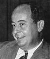
In the 1950's, Von Neumann came up with the idea whilst working on a
suggestion from his friend Ulam (a mathematician) as to how to construct
a computer program capable of self-reproduction.
|
|
Analysis of Cellular Automata
|
The properties of dynamical systems such as CA's may be loosely characterized
by referring to their long term behaviour:
- Strange Attractor: System behaves chaotically for all eternity.
- Limit Cycle: System falls into an infinite loop.
- Fixed Point / Limit Point: System halts.
To relate these general principles of dynamical systems to CA's, Wolfram
classifies CA's as follows:
- Moves into a homogeneous state
- limit point
- Moves into simple, separated, periodic structures
- limit cycle
- Produces chaotic aperiodic patterns
- strange attractors
- Produces complex patterns of localized structures
- virtual life?!
|
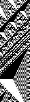
The Game of Life
by John Conway
- Eight-neighbourhood grid
- Two-state FSM's (ON or OFF)
Rules for transition table...
if (cell is OFF)
{
if(exactly 3 neighbours are ON) cell turns ON
else cell stays OFF
}
if (cell is ON)
{
if (2 or 3 neighbours are ON) cell stays ON
else cell turns OFF
}
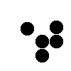
Some common formations...

|

|

|
|
| Spinner
(animated) |
1 |
2 |
1 |

|
|
|
|
|
|
| Glider
(animated) |
1 |
2 |
3 |
4 |
1 |
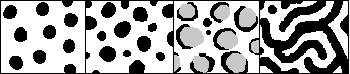
2. Reaction-Diffusion Systems
(RD)
|
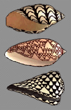
RD-generated shell patterns
(Fowler, Meinhardt, Prusinkiewicz 1992)
|
References:
A. Turing,
"The Chemical Basis of Morphogenesis",
Philosophical Transactions of the Royal Society, Vol. 237, pp37-72, August
14, 1952
J. Cohen, I. Stewart,
"Let T equal tiger",
New Scientist, pp40-44, 6 Nov 1993
G. Turk,
"Generating Textures on Arbitrary Surfaces Using Reaction - Diffusion",
SIGGRAPH proceedings, pp289-298, 1991
|
What is a Reaction-Diffusion system?
- Chemicals reacting with each other as they diffuse through tissue in living
systems may be partially responsible for the formation of some patterns in
the morphology of living things...
...these hypothetical chemicals are called morphogens.
- The concentration of chemicals diffusing through tissue may be modelled
using a set of PDE's which may be solved using finite-difference methods.
- Such a system is a 'reaction-diffusion' system. (The morphogens react
with one another as they diffuse through the tissue.)
Where'd the idea come from?
|
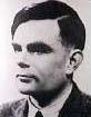
Alan Turing in 1952 proposed the RD mechanism as a means of explaining
cell-differentiation during embryonic development.
At this stage in the history of Developmental Biology, the evidence to
demonstrate that RD systems do occur in natural systems is largely
circumstantial (but quite convincing).
|
|
Analysis of RD Systems.
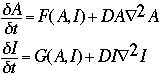
The simplest RD system has two reacting chemicals:
- Activator (concentration A)
- Inhibitor (concentration I)
These diffuse through a space at different rates:
The change of A and I over time varies with the sum of:
- A function (F or G) of the concentrations at that point.
- The rate of diffusion of the activator or inhibitor (DA or DI)
multiplied by a measure of the concentration gradient at that point as given
by the Laplacian for A or I. (Refer to Mathworld for Del
and the Vector Laplacian)
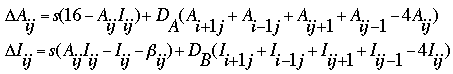
Using RD for Pattern Formation
- Perform an RD simulation on a 2D grid.
- Chemicals diffuse between cells across shared boundaries.
For example:
- Commence simulation with an irregularity in the chemical concentration (denoted Beta).
- The Laplacian is calculated above by summing the concentrations
of a cell (i,j)'s four neighbours (giving them equal weighting since
the shared edge across which diffusion occurs is, in our regular
grid, always equal) and subtracting four times the concentration
of the chemical at the cell(i,j).
More interesting results
- Vary the value of s or change the rates of diffusion of the chemicals
for different results.
- Have multiple chemicals diffusing and reacting.
- Can have one RD system lay down a stable initial pattern and then:
|
- Run another simulation over the top of that one, using the first pattern
as a non-random seed
- Freeze part of the initial pattern and run the second simulation in
the unfrozen portion
- Use the initial pattern to non-uniformly vary the rate of diffusion
of chemicals in the second simulation
- Vary the diffusion rate across different portions of the grid or run
the simulation on irregular grids
|
|
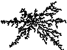
An alternative (and fascinating!) set of reactions is known as the Gray-Scott RD system (applet, pre-rendered movies).
3. Diffusion Limited Aggregation
(DLA) & Diffusion Limited Accretive Growth
|
References:
Kaandorp, J.A.,
"Fractal Modelling: Growth and Form in Biology",
Springer-Verlag, 1994
Meakin, P.,
"A new model for biological pattern formation"
J. Theor. Biol. 118 pp101-113, 1986
|
What is Diffusion Limited Aggregation?
DLA is a discrete model of Diffusion Limited Accretive Growth...
- This is growth by expansion along a structure's border at a
rate governed by the gradient of consumable nutrient in the medium
surrounding the structure.
- DLA simulates the diffusion of nutrients through a medium by random
movements of particles across a grid.
- The growing structure is seeded by a (central) fixed cell.
- Once a randomly moving particle hits the growing structure, it sticks there
permanently.
Diffusion Limited Accretive Growth has been used to model:
- Growth of bacteria on an agar plate
- Development of corals and sponges
- The discrete model (DLA) correctly reproduces the behaviour of metallic
ions as they are deposited on an electrode but ignores the active,
nutrient-consuming role of a living organism
|
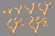
A model of the sponge Haliclona occulata
(Kaandorp, 1992)
|
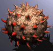
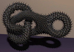
4. Cellular Texture Generation
References:
Fleischer K.W. et al,
"Cellular Texture Generation",
SIGGRAPH proceedings, p239-248, 1995
(All images below by Fleischer '95)
|
- Cellular textures are surface textures with 3D geometry, orientation
and colour
- The method utilizes elements of particle systems, developmental models
and reaction-diffusion systems
- Cells are modelled as particles in a continuous medium
- Cells may release or respond to chemicals diffusing through the continuous
medium
|
Cells act in a space as determined by cell programs with parameters governed
by the local conditions experienced by the cell
|
Cells may (for example):
- Collide with and adhere to other structures and each other
- Absorb/release chemicals from/to the medium & adjacent cells
- Divide to produce daughter cells
- Be constrained to move on a surface
|
|
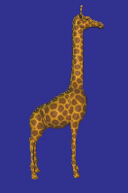
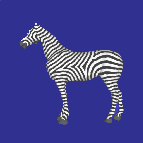
Cells have been represented visually as oriented and differentiated:
- plant thorns
- reptile scales
- animal fur
|
|
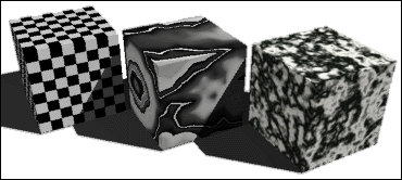
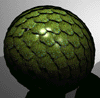
5. Generating Solid Textures
(Lovely Checks, Gentle Wood-Grains and Gorgeous Marbles)
References:
Perlin, K.,
"An Image Synthesizer"
SIGGRAPH proceedings, Vol.19, No.3, 1985, pp287-296
Watt, Watt,
"Advanced Animation and Rendering Techniques"
Addision Welsey, 1992, pp205-211
Foley, van Dam, Feiner, Hughes,
"Computer Graphics, Principles and Practice"
2nd edn, Addison-Wesley, 1987, pp1015-1018
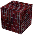
Why bother with textures?
- The addition of surface textures to a geometric model improves realism.
- Textures may be used to disguise the starkness typical of computer graphics by faking:
- Geometry (windows, bricks, panels, rivets)
- Surface detail (stains, rust, graffiti, mosaics, fresco)
- Material properties (marble, timber, concrete, steel, cloth)
...these benefits come without the added expense (rendering & storage) of
extra geometry.
What is a solid texture?
A model may be textured by mapping a 2D image over its surface.
Imagine pasting patterned paper on the model (or gift-wrapping it) and you have
the idea.
Or...
...a model may be textured according to the location of its geometry in 3-space
using a volumetric/solid/3D texture.
Imagine carving the model out of solid timber or a block of marble. The grain
in the timber or veins of the marble will of course pattern the final object!
2D, non-procedural textures are:
- Easy to produce (scanned drawing, photograph etc.)
- Difficult to map (without distortions) over geometry of non-uniform curvature
- Difficult to map over complex topologies
- Of constant resolution
- Frequently 'tiled' to avoid pixellation by over-enlargement.
This results in pattern artefacts under some circumstances.
(In other circumstances this is desirable eg. house-bricks, paving stones)
3D, procedural textures are:
- Difficult to produce to arbitrary specifications
- Naturally calculated for arbitrary curvatures
- Naturally calculated for arbitrary topologies
- Of potentially infinite resolution (no pixellation)
- Of potentialy infinite expanse (no need to tile)
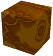
A Wood-Grain (Solid) Texture
Create a solid colour-map made from concentric cylinders of varying colours
(e.g. browns):
- For the best effects, angle the model to be textured so that its major axis
cuts slightly across the axis of the cylinders
- Perturb the cylinders' radii slightly
- Twist the cylinders longitudinally
A Marble (Solid) Texture
- Noise:
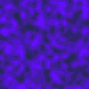
|
- Define a regular lattice of points indexed by integers
- Assign a random value to each lattice point
- The noise value at a lattice point is its random value
- The noise value between lattice points is computed by interpolation
(e.g. linear or cubic)
|
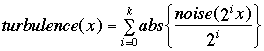
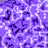
- Turbulence:
- The turbulence function takes a position x and returns a scalar:
where k is the smallest integer satisfying:
- The turbulence function sums calls to the noise function to give statistically
identical detail at various resolutions.
(Note similarity to the refinement of midpoint perturbation in the production
of fractal mountains.)
- Veins:
|
- Regular veins of material may be described by a sin wave
- Pass the sin wave through a colour map (map scalar to intensity/colour
using a spline):
marble(x) = marble_colour(sin(x))
- Add turbulence to perturb the regularity:
marble(x) = marble_colour(sin(x+turbulence(x)))
|
lecture notes | home
All material accessed from www.cs(se).monash.edu.au/~cema
is
© Copyright 1994-2008 Alan Dorin, Jon McCormack & Monash University except where noted.